Livestock

Livestock population

The principal variable characterizing the livestock production in GLOBIOM is the number of animals by species, production system and production type in each Simulation Unit. GLOBIOM differentiates four species aggregates: cattle and buffaloes (bovines), sheep and goats (small ruminants), pigs, and poultry. Eight production systems are specified for ruminants: grazing systems in arid (LGA), humid (LGH) and temperate/highland areas (LGT); mixed systems in arid (MXA), humid (MXH) and temperate/highland areas (MXT); urban systems (URB); and other systems (OTH). Mixed systems are an aggregate of the more detailed original Sere and Steinfeld’s classes (Sere and Steinfeld, 1996 [103]) – mixed rainfed and mixed irrigated. Two production systems are specified for monogastrics: smallholders (SMH) and industrial systems (IND). In terms of production type, dairy and meat herds are modeled separately for ruminants: dairy herd includes adult females and replacement heifers, whose diets are distinguished. Poultry in smallholder systems is considered as mixed producer of meat and eggs, and poultry in industrial systems is split into laying hens and broilers, with differentiated diet regimes. Overall livestock numbers at the country level are, where possible while respecting minimum herd dynamics rules, harmonized with FAOSTAT.

The spatial distribution of ruminants and their allocation between production systems follows an updated version of Wint and Robinson (Wint and Robinson, 2007 [112]). Since better information is not available, it is assumed that the share of dairy and meat herds within one region is the same in all production systems. The share is obtained from the FAO country level data about milk producing animals and total herd size. Monogastrics are not treated in a spatially explicit way since no reliable maps are currently available, and because monogastrics are not linked in the model to specific spatial features, like grasslands. The split between smallholder and industrial systems follows Herrero et al. (2013) [27].

Livestock products

Each livestock category is characterized by product yield, feed requirements, and a set of direct GHG emission coefficients. On the output side, seven products are defined: bovine meat and milk, small ruminant meat and milk, pig meat, poultry meat, and eggs. For each region, production type and production system, individual productivities are determined.

Bovine and small ruminant productivities are estimated through the RUMINANT model (Herrero et al., 2008 [28]; Herrero et al., 2013 [27]), in a three steps process which consists of first, specifying a plausible feed ration; second, calculating in RUMINANT the corresponding yield; and finally confronting at the region level with FAOSTAT (Supply Utilization Accounts) data on production. These three steps were repeated in a loop until a match with the statistical data was obtained. Monogastrics productivities were disaggregated from FAOSTAT based on assumptions about potential productivities and the relative differences in productivities between smallholder and industrial systems. The full detail of this procedure is provided in Herrero et al. (2013) [27].

Final livestock products are expressed in primary commodity equivalents. Each product is considered as a differentiated good with a specific market except for bovine and small ruminant milk that are merged in a single milk market. The two milk types are therefore treated as perfect substitutes.

Livestock feed

Feed requirements for ruminants are computed simultaneously with the yields (Herrero et al., 2013 [27]). Specific diets are defined for the adult dairy females, and for the other animals. The feed requirements are first calculated at the level of four aggregates – grains (concentrates), stover, grass, and other. When estimating the feed-yield couples, the RUMINANT model takes into account different qualities of these aggregates across regions and systems. Feed requirements for monogastrics are at this level determined through literature review presented in Herrero et al. (2013) [27]. In general, it is assumed that in industrial systems pigs and poultry consume 10 and 12 kg dry matter of concentrates per TLU and day, respectively, and concentrates are the only feed sources. Smallholder animals get only one quarter of the amount of grains fed in industrial systems, the rest is supposed to come from other sources, like household waste, not explicitly represented in GLOBIOM.

The aggregate GRAINS input group is harmonized with feed quantities as reported at the country level in Commodity Balances of FAOSTAT. The harmonization proceeds in two steps, where first, GRAINS in the feed rations are adjusted so that total feed requirements at the country level match with total feed quantity in Commodity Balances, and second, “Grains” is disaggregated into 11 feed groups: Barley, Corn, Pulses, Rice, Sorghum & Millet, Soybeans, Wheat, Cereal Other, Oilseed Other, Crops Other, Animal Products. The adjustment of total GRAINS quantities is first done through shifts between the GRAINS and OTHER categories in ruminant systems. Hence, if total GRAINS are lower than the statistics, a part or total feed from the OTHER category is moved to GRAINS. If this is not enough, all GRAINS requirements of ruminants are shifted up in the same proportions. If total GRAINS are higher than the statistics, then firstly a part of them must be reallocated to the OTHER category. If this is not enough, values are to be kept, which then results in higher GRAINS demand than reported in FAOSTAT. This inconsistency is overcome in GLOBIOM, by creating a “reserve” of the missing GRAINS. This reserve is in simulations kept constant, thus it enables to reproduce the base year activity levels mostly consistent with FAOSTAT, but requires that all additional GRAINS demand arising over the simulation horizon is satisfied from real production. The decomposition of GRAINS into the 11 subcategories has to follow predefined minima and maxima of the shares of feedstuffs in a ration differentiated by species and region. At the same time, the shares of the feedstuffs corresponding to country level statistics need to be respected. This problem is solved as minimization of the square deviations from the prescribed minimum and maximum limits. In GLOBIOM, the balance between demand and supply of the crop products entering the GRAINS subcategories needs to be satisfied at regional level. Substitution ratios are defined for the byproducts of biofuel industry so that they can also enter the feed supply.

STOVER is supposed less mobile than GRAINS, therefore stover demand in GLOBIOM is forced to match supply at grid level. The demand is mostly far below the stover availability. In the cells where this is not the case, the same system of reserve is implemented as for the grains. No adjustments are done to the feed rations as such.

There are unfortunately no worldwide statistics available on either consumption or production of grass. Hence grass requirements were entirely based on the values calculated with RUMINANT, and were used to estimate the grassland extent and productivity. (This procedure is described in the next section.)

Finally, the feed aggregate OTHER is represented in a simplified way, where it is assumed that it is satisfied entirely from a reserve in the base year, and all additional demand needs to be satisfied by forage production on grasslands.

Grazing forage availability

The demand and supply of grass need to match at the level of Simulation Unit in GLOBIOM. But reliable information about grass forage supply is not available even at the country level. The forage supply is a product of the utilized grassland area and of forage productivity. However, at global scale, Ramankutty et al. (2008) [77] estimated that the extent of pastures spans in the 90% confidence interval between 2.36 and 3.00 billion hectares. The FAOSTAT estimate of 3.44 billion hectares itself falls outside of this interval which illustrates the level of uncertainty in the grassland extent. Similarly, with respect to forage productivity, different grassland production models perform better for different forage production systems and all are confronted with considerable uncertainty due to limited information about vegetation types, management practices, etc. (Conant and Paustian, 2004 [8]). These limitations precluded reliance on any single source of information or output from a single model. Therefore three different grass productivity sources were considered: CENTURY on native grasslands, CENTURY on native and managed grasslands, and EPIC on managed grasslands.

A systematic process was developed for selecting the suitable productivity source for each of GLOBIOM’s 30 regions. This process allowed reliance on sound productivity estimates that are consistent with other GLOBIOM datasets like spatial livestock distribution and feed requirements. Within this selection process, the area of utilized grasslands corresponding to the base year 2000 was determined simultaneously with the suitable forage productivity layer. Two selection criteria were used: livestock requirements for forage and area of permanent meadows and pastures from FAOSTAT. The selection process was based on simultaneous minimization of i) the difference between livestock demand for forage and the model-estimates of forage supply and ii) the difference between the utilized grassland area and FAOSTAT statistics on permanent meadows and pastures. Regional differentiation in grassland management intensity, ranging from dry grasslands with minimal inputs to mesic, planted pastures that are intensively managed with large external inputs – further informed the model selection by enabling constraints in the number of models for dry grasslands.

To calculate the utilized grassland area, the potential grassland area was first defined as the area belonging to one of the following GLC2000 land cover classes: 13 (Herbaceous Cover, closed-open), 16-18 (Cultivated and managed areas, Mosaic: Cropland / Tree Cover / Other natural vegetation, Mosaic: Cropland / Shrub and/or grass cover), excluding area identified as cropland according to the IFPRI crop distribution map (You and Wood, 2006 [113]), and 11, 12, 14 (Shrub Cover, closed-open, evergreen, Shrub Cover, closed-open, deciduous, Sparse herbaceous or sparse shrub cover). In each Simulation Unit the utilized area was calculated by dividing total forage requirements by forage productivity. In Simulation Units where utilized area was smaller than the potential grassland area, the difference would be allocated to either “Other Natural Land” or “Other Agricultural Land” depending on the underlying GLC2000 class. In Simulation Units where the grassland area necessary to produce the forage required in the base year was larger than the potential grassland area, a “reserve” was created to ensure base year feasibility, but all the additional grass demand arising through future livestock production increases needed to be satisfied from grasslands.

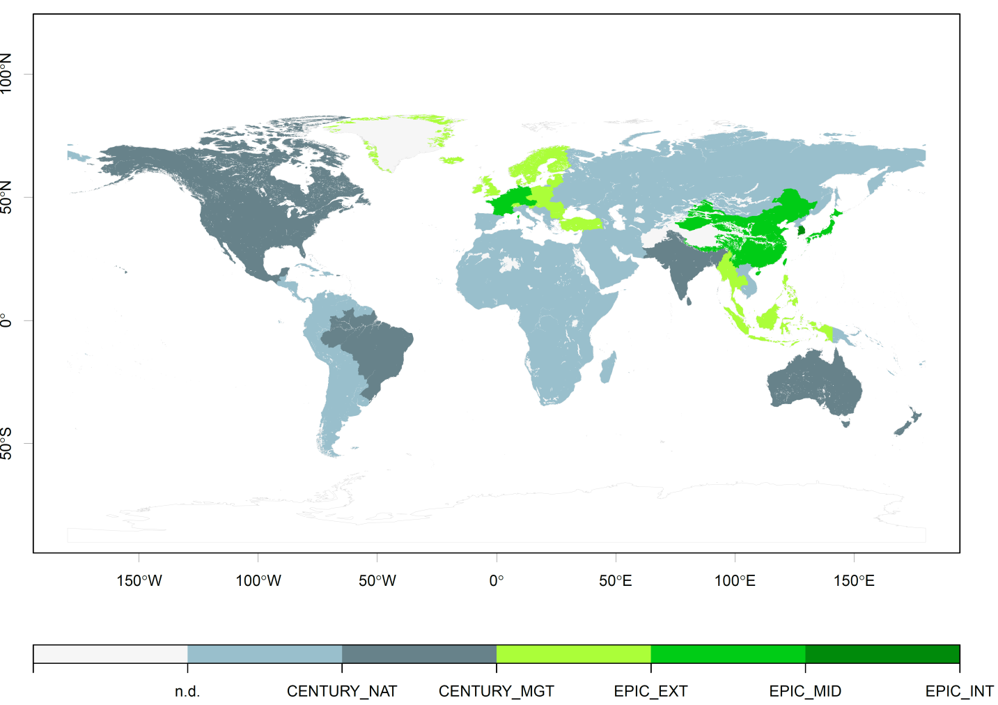
Fig. 20 Data sources used to parameterize forage availability in different world regions. CENTURY_NAT – CENTURY model for native grasslands; CENTURY_MGT – CENTURY model for productive grasslands; EPIC_EXT – EPIC model for grasslands under extensive management; EPIC_MID – EPIC model for grasslands under semi-intensive management; EPIC_INT – EPIC model for grasslands under intensive management.

Forage productivity was estimated using the CENTURY (Parton et al., 1987 [72]; Parton et al., 1993 [71]) and EPIC (Williams and Singh, 1995 [111]) models. The CENTURY model was run globally at 0.5 degree resolution to estimate native forage and browse and planted pastures productivity. It was initiated with 2000 year spin-ups using mean monthly climate from the Climate Research Unit (CRU) of the University of East Anglia with native vegetation for each grid cell, except cells dominated by rock, ice, and water, which were excluded. Information about native vegetation was derived from the Potsdam intermodal comparison study (Schloss et al., 1999 [99]). Plant community and land management (grazing) was based on growing-season grazing and 50 per cent forage removal. Areas under native vegetation that were grazed were identified using the map of native biomes subject to grazing and subtracting estimated crop area within those biomes in 2006 (Ramankutty et al., 2008 [77]). It is assumed 50 per cent grazing efficiency for grass, and 25 per cent for browse for native grasslands. These CENTURY-based estimates of native grassland forage production (CENTURY_NAT) were used for most regions with low-productivity grasslands (Fig. 20).

Both the CENTURY and EPIC models were used to estimate forage production in mesic, more productive regions. For the CENTURY model, forage yield was simulated using a highly-productive, warm-season grass parameterization. Production was modeled in all cells and applied to areas of planted pasture, which were estimated based on biomes that were not native rangelands, but were under pasture in 2006 according to Ramankutty (Ramankutty et al., 2008 [77]). Pastures were replanted in the late winter every ten years, with grazing starting in the second year. Observed monthly precipitation and minimum and maximum temperatures between 1901 and 2006 were from the CRU Time Series data, CRU TS30 (Mitchell and Jones, 2005 [63]) Soils data were derived from the FAO Soil Map of the World, as modified by Reynolds et al. (2000) [83]. CENTURY model output for productive pastures (CENTURY_MGT) were the best-match for area/forage demand in much of the world with a mixture of mesic and drier pastures.

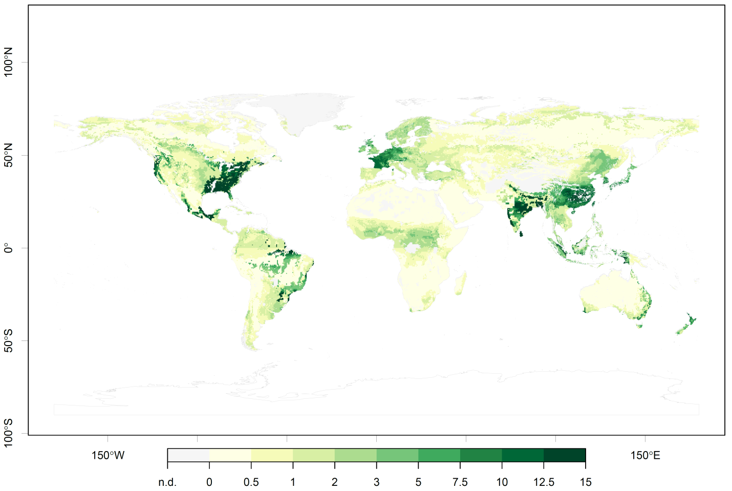
Fig. 21 Forage available for livestock in tonnes of dry matter per hectare as the result of combination of outputs from the CENTURY and EPIC models.

The EPIC model was the best fit for much of Europe and Eastern Asia, where most of the forage production is in intensively-managed grasslands. The EPIC simulations used the same soil and climatic drivers as the CENTURY runs plus topography data (high-resolution global Shuttle Radar Topography Mission digital elevation model (SRTM) and the Global 30 Arc Second Elevation Data (GTOPO30). Warm and cold seasonal grasses were simulated in EPIC, and the simulations included a range of management intensities represented by different levels of nitrogen fertilizer inputs and off-take rates. The most intensive management minimizing nitrogen stress and applying 80% off-take rates (EPIC_INT) was found to be the best match for South Korea. Highly fertilized grasslands but with an off-take rate of 50% only were identified in Western Europe, China and Japan (EPIC_MID), and finally extensive management, only partially satisfying the nitrogen requirements and considering 20% off-take rates corresponded best to Central and Northern Europe and South-East Asia (EPIC_EXT). The resulting hybrid forage availability map is represented in Fig. 21.

Livestock dynamics

In general, the number of animals of a given species and production type in a particular production system and Supply Unit is an endogenous variable. This means that it will decrease or increase in relation to changes in demand and the relative profitability with respect to competing activities.

Herd dynamics constraints need however to be respected. First, dairy herds are constituted of adult females and followers, and expansion therefore occurs in predefined proportions in the two groups. Moreover, for regions where the specialized meat herds are insignificant (no suckler cows), expansion of meat animals (surplus heifers and males) is also assumed proportional in size to the dairy herd. The ruminants in urban systems are not allowed to expand because this category is not well known and because it is fairly constrained by available space in growing cities. Finally, the decrease of animals per system and production type higher than 15 per cent per 10 years period are not considered, and no increase by more than 100 per cent on the same period. At the level of individual systems, the decrease can however be as deep as 50 per cent per system on a single period.

For monogastrics, the assumption is made that all additional supply will come from industrial systems and hence the number of animals in other systems is kept constant (Keyzer et al., 2005 [42]).