Note
This page is generated from inline documentation in MESSAGE/model_core.gms.
MESSAGE core formulation
The MESSAGEix systems-optimization model minimizes total costs while satisfying given demand levels for commodities/services and considering a broad range of technical/engineering constraints and societal restrictions (e.g. bounds on greenhouse gas emissions, pollutants, system reliability). Demand levels are static (i.e. non-elastic), but the demand response can be integrated by linking MESSAGEix to the single sector general-economy MACRO model included in this framework.
For the complete list of sets, mappings and parameters, refer to the auto-documentation page Sets and mappings and Parameter definition. The mathematical notation that is used to represent sets and mappings in the equations below can also be found in the tables in Sets and mappings.
Variable definitions
Decision variables
Variable |
Explanatory text |
|---|---|
\(OBJ \in \mathbb{R}\) |
Objective value of the optimization program |
\(EXT_{n,c,g,y} \in \mathbb{R}_+\) |
Extraction of non-renewable/exhaustible resources from reserves |
\(STOCK_{n,c,l,y} \in \mathbb{R}_+\) |
Quantity in stock (storage) at start of period \(y\) |
\(STOCK\_CHG_{n,c,l,y,h} \in \mathbb{R}\) |
Input or output quantity into intertemporal commodity stock (storage) |
\(COST\_NODAL_{n,y} \in \mathbb{R}\) |
System costs at the node level over time |
\(REN_{n,t,c,g,y,h} \in \mathbb{R}_+\) |
Activity of renewable technologies per grade |
\(CAP\_NEW_{n,t,y} \in \mathbb{R}_+\) |
Newly installed capacity (yearly average over period duration) |
\(CAP_{n,t,y^V,y} \in \mathbb{R}_+\) |
Maintained capacity in year \(y\) of vintage \(y^V\) |
\(CAP\_FIRM_{n,t,c,l,y,q} \in \mathbb{R}_+\) |
Capacity counting towards firm (dispatchable) |
\(ACT_{n,t,y^V,y,m,h} \in \mathbb{R}\) |
Activity of a technology (by vintage, mode, subannual time) |
\(ACT\_RATING_{n,t,y^V,y,c,l,h,q} \in \mathbb{R}_+\) |
Auxiliary variable for activity attributed to a particular rating bin 1 |
\(CAP\_NEW\_UP_{n,t,y} \in \mathbb{R}_+\) |
Relaxation of upper dynamic constraint on new capacity |
\(CAP\_NEW\_LO_{n,t,y} \in \mathbb{R}_+\) |
Relaxation of lower dynamic constraint on new capacity |
\(ACT\_UP_{n,t,y,h} \in \mathbb{R}_+\) |
Relaxation of upper dynamic constraint on activity 2 |
\(ACT\_LO_{n,t,y,h} \in \mathbb{R}_+\) |
Relaxation of lower dynamic constraint on activity 2 |
\(LAND_{n,s,y} \in [0,1]\) |
Relative share of land-use scenario (for land-use model emulator) |
\(EMISS_{n,e,\widehat{t},y} \in \mathbb{R}\) |
Auxiliary variable for aggregate emissions by technology type |
\(REL_{r,n,y} \in \mathbb{R}\) |
Auxiliary variable for left-hand side of relations (linear constraints) |
\(COMMODITY\_USE_{n,c,l,y} \in \mathbb{R}\) |
Auxiliary variable for amount of commodity used at specific level |
\(COMMODITY\_BALANCE_{n,c,l,y,h} \in \mathbb{R}\) |
Auxiliary variable for right-hand side of Auxiliary COMMODITY_BALANCE |
\(STORAGE_{n,t,l,c,y,h} \in \mathbb{R}\) |
State of charge or content of storage at each sub-annual timestep |
\(STORAGE\_CHARGE_{n,t,l,c,y,h} \in \mathbb{R}\) |
Charging of storage in each sub-annual timestep (negative for discharging) |
The index \(y^V\) is the year of construction (vintage) wherever it is necessary to clearly distinguish between year of construction and the year of operation.
All decision variables are by year, not by (multi-year) period, except \(STOCK_{n,c,l,y}\). In particular, the new capacity variable \(CAP\_NEW_{n,t,y}\) has to be multiplied by the number of years in a period \(|y| = duration\_period_{y}\) to determine the available capacity in subsequent periods. This formulation gives more flexibility when it comes to using periods of different duration (more intuitive comparison across different periods).
The current model framework allows both input or output normalized formulation. This will affect the parametrization, see Section Efficiency - output- vs. input defined technologies for more details.
Auxiliary variables
Variable |
Explanatory text |
|---|---|
\(DEMAND_{n,c,l,y,h} \in \mathbb{R}\) |
Demand level (in equilibrium with MACRO integration) |
\(PRICE\_COMMODITY_{n,c,l,y,h} \in \mathbb{R}\) |
Commodity price (undiscounted marginals of Equation COMMODITY_BALANCE_GT and Equation COMMODITY_BALANCE_LT) |
\(PRICE\_EMISSION_{n,\widehat{e},\widehat{t},y} \in \mathbb{R}\) |
Emission price (undiscounted marginals of Equation EMISSION_CONSTRAINT) |
\(COST\_NODAL\_NET_{n,y} \in \mathbb{R}\) |
System costs at the node level net of energy trade revenues/cost |
\(GDP_{n,y} \in \mathbb{R}\) |
Gross domestic product (GDP) in market exchange rates for MACRO reporting |
Objective function
The objective function of the MESSAGEix core model
Equation OBJECTIVE
The objective function (of the core model) minimizes total discounted systems costs including costs for emissions, relaxations of dynamic constraints
Regional system cost accounting function
Accounting of regional system costs over time
Equation COST_ACCOUNTING_NODAL
Accounting of regional systems costs over time as well as costs for emissions (taxes), land use (from the model land-use model emulator), relaxations of dynamic constraints, and linear relations.
Here, \(n^L \in N(n)\) are all nodes \(n^L\) that are sub-nodes of node \(n\). The subset of technologies \(t \in T(\widehat{t})\) are all tecs that belong to category \(\widehat{t}\), and similar notation is used for emissions \(e \in E\).
Resource and commodity section
Constraints on resource extraction
Equation EXTRACTION_EQUIVALENCE
This constraint translates the quantity of resources extracted (summed over all grades) to the input used by all technologies (drawing from that node). It is introduced to simplify subsequent notation in input/output relations and nodal balance constraints.
\[\begin{split}\sum_{g} EXT_{n,c,g,y} = \sum_{\substack{n^L,t,m,h,h^{OD} \\ y^V \leq y \\ \ l \in L^{RES} \subseteq L }} input_{n^L,t,y^V,y,m,n,c,l,h,h^{OD}} \cdot ACT_{n^L,t,m,y,h}\end{split}\]
The set \(L^{RES} \subseteq L\) denotes all levels for which the detailed representation of resources applies.
Equation EXTRACTION_BOUND_UP
This constraint specifies an upper bound on resource extraction by grade.
\[EXT_{n,c,g,y} \leq bound\_extraction\_up_{n,c,g,y}\]
Equation RESOURCE_CONSTRAINT
This constraint restricts that resource extraction in a year guarantees the “remaining resources” constraint, i.e., only a given fraction of remaining resources can be extracted per year.
\[\begin{split}EXT_{n,c,g,y} \leq resource\_remaining_{n,c,g,y} \cdot \Big( & resource\_volume_{n,c,g} \\ & - \sum_{y' < y} duration\_period_{y'} \cdot EXT_{n,c,g,y'} \Big)\end{split}\]
Equation RESOURCE_HORIZON
This constraint ensures that total resource extraction over the model horizon does not exceed the available resources.
\[\sum_{y} duration\_period_{y} \cdot EXT_{n,c,g,y} \leq resource\_volume_{n,c,g}\]
Constraints on commodities and stocks
Auxiliary COMMODITY_BALANCE
For the commodity balance constraints below, we introduce an auxiliary variable called \(COMMODITY\_BALANCE\). This is implemented
as a GAMS $macro function.
\[\begin{split}\sum_{\substack{n^L,t,m,h^A \\ y^V \leq y}} output_{n^L,t,y^V,y,m,n,c,l,h^A,h} \cdot duration\_time\_rel_{h,h^A} \cdot ACT_{n^L,t,y^V,y,m,h^A} & \\ - \sum_{\substack{n^L,t,m,h^A \\ y^V \leq y}} input_{n^L,t,y^V,y,m,n,c,l,h^A,h} \cdot duration\_time\_rel_{h,h^A} \cdot ACT_{n^L,t,m,y,h^A} & \\ + \ STOCK\_CHG_{n,c,l,y,h} + \ \sum_s \Big( land\_output_{n,s,y,c,l,h} - land\_input_{n,s,y,c,l,h} \Big) \cdot & LAND_{n,s,y} \\[4pt] - \ demand\_fixed_{n,c,l,y,h} = COMMODITY\_BALANCE_{n,c,l,y,h} \quad \forall \ l \notin (L^{RES}, & L^{REN}, L^{STOR} \subseteq L)\end{split}\]
The commodity balance constraint at the resource level is included in the Equation RESOURCE_CONSTRAINT, while at the renewable level, it is included in the Equation RENEWABLES_EQUIVALENCE, and at the storage level, it is included in the Equation STORAGE_BALANCE.
Equation COMMODITY_BALANCE_GT
This constraint ensures that supply is greater or equal than demand for every commodity-level combination.
\[COMMODITY\_BALANCE_{n,c,l,y,h} \geq 0\]
Equation COMMODITY_BALANCE_LT
This constraint ensures that the supply is smaller than or equal to the demand for all commodity-level combinations given in the \(balance\_equality_{c,l}\). In combination with the constraint above, it ensures that supply is (exactly) equal to demand.
\[COMMODITY\_BALANCE_{n,c,l,y,h} \leq 0\]
Equation STOCKS_BALANCE
This constraint ensures the inter-temporal balance of commodity stocks. The parameter \(commodity\_stocks_{n,c,l}\) can be used to model exogenous additions to the stock
\[\begin{split}STOCK_{n,c,l,y} + commodity\_stock_{n,c,l,y} = duration\_period_{y} \cdot & \sum_{h} STOCK\_CHG_{n,c,l,y,h} \\ & + STOCK_{n,c,l,y+1}\end{split}\]
Technology section
Technical and engineering constraints
The first set of constraints concern technologies that have explicit investment decisions and where installed/maintained capacity is relevant for operational decisions. The set where \(T^{INV} \subseteq T\) is the set of all these technologies.
Equation CAPACITY_CONSTRAINT
This constraint ensures that the actual activity of a technology at a node cannot exceed available (maintained) capacity summed over all vintages, including the technology capacity factor \(capacity\_factor_{n,t,y,t}\).
\[\sum_{m} ACT_{n,t,y^V,y,m,h} \leq duration\_time_{h} \cdot capacity\_factor_{n,t,y^V,y,h} \cdot CAP_{n,t,y^V,y} \quad \forall \ t \ \in \ T^{INV}\]
Equation CAPACITY_MAINTENANCE_HIST
The following three constraints implement technology capacity maintenance over time to allow early retirment. The optimization problem determines the optimal timing of retirement, when fixed operation-and-maintenance costs exceed the benefit in the objective function.
The first constraint ensures that historical capacity (built prior to the model horizon) is available as installed capacity in the first model period.
\[\begin{split}CAP_{n,t,y^V,'first\_period'} & \leq remaining\_capacity_{n,t,y^V,'first\_period'} \cdot duration\_period_{y^V} \cdot historical\_new\_capacity_{n,t,y^V} \\ & \text{if } y^V < 'first\_period' \text{ and } |y| - |y^V| < technical\_lifetime_{n,t,y^V} \quad \forall \ t \in T^{INV}\end{split}\]
Equation CAPACITY_MAINTENANCE_NEW
The second constraint ensures that capacity is fully maintained throughout the model period in which it was constructed (no early retirement in the period of construction).
\[CAP_{n,t,y^V,y^V} = remaining\_capacity_{n,t,y^V,y^V} \cdot duration\_period_{y^V} \cdot CAP\_NEW_{n,t,y^V} \quad \forall \ t \in T^{INV}\]
The current formulation does not account for construction time in the constraints, but only adds a mark-up to the investment costs in the objective function.
Equation CAPACITY_MAINTENANCE
The third constraint implements the dynamics of capacity maintenance throughout the model horizon. Installed capacity can be maintained over time until decommissioning, which is irreversible.
\[\begin{split}CAP_{n,t,y^V,y} & \leq remaining\_capacity_{n,t,y^V,y} \cdot CAP_{n,t,y^V,y-1} \\ \quad & \text{if } y > y^V \text{ and } y^V > 'first\_period' \text{ and } |y| - |y^V| < technical\_lifetime_{n,t,y^V} \quad \forall \ t \in T^{INV}\end{split}\]
Equation OPERATION_CONSTRAINT
This constraint provides an upper bound on the total operation of installed capacity over a year. It can be used to represent reuqired scheduled unavailability of installed capacity.
\[\sum_{m,h} ACT_{n,t,y^V,y,m,h} \leq operation\_factor_{n,t,y^V,y} \cdot capacity\_factor_{n,t,y^V,y,m,\text{'year'}} \cdot CAP_{n,t,y^V,y} \quad \forall \ t \in T^{INV}\]
This constraint is only active if \(operation\_factor_{n,t,y^V,y} < 1\).
Equation MIN_UTILIZATION_CONSTRAINT
This constraint provides a lower bound on the total utilization of installed capacity over a year.
\[\sum_{m,h} ACT_{n,t,y^V,y,m,h} \geq min\_utilization\_factor_{n,t,y^V,y} \cdot CAP_{n,t,y^V,y} \quad \forall \ t \in T^{INV}\]
This constraint is only active if \(min\_utilization\_factor_{n,t,y^V,y}\) is defined.
Constraints representing renewable integration
Equation RENEWABLES_EQUIVALENCE
This constraint defines the auxiliary variables \(REN\) to be equal to the output of renewable technologies (summed over grades).
\[\begin{split}\sum_{g} REN_{n,t,c,g,y,h} \leq \sum_{\substack{n,t,m,l,h,h^{OD} \\ y^V \leq y \\ \ l \in L^{REN} \subseteq L }} input_{n^L,t,y^V,y,m,n,c,l,h,h^{OD}} \cdot ACT_{n^L,t,m,y,h}\end{split}\]
The set \(L^{REN} \subseteq L\) denotes all levels for which the detailed representation of renewables applies.
Equation RENEWABLES_POTENTIAL_CONSTRAINT
This constraint sets the potential potential by grade as the upper bound for the auxiliary variable \(REN\).
\[\begin{split}\sum_{\substack{t,h \\ \ t \in T^{R} \subseteq t }} REN_{n,t,c,g,y,h} \leq \sum_{\substack{l \\ l \in L^{R} \subseteq L }} renewable\_potential_{n,c,g,l,y}\end{split}\]
Equation RENEWABLES_CAPACITY_REQUIREMENT
This constraint connects the capacity factor of a renewable grade to the installed capacity of a technology. It sets the lower limit for the capacity of a renewable technology to the summed activity over all grades (REN) devided by the capactiy factor of this grade. It represents the fact that different renewable grades require different installed capacities to provide their full potential.
\[\begin{split}\sum_{y^V, h} & CAP_{n,t,y^V,y} \cdot operation\_factor_{n,t,y^V,y} \cdot capacity\_factor_{n,t,y^V,y,h} \\ & \quad \geq \sum_{g,h,l} \frac{1}{renewable\_capacity\_factor_{n,c,g,l,y}} \cdot REN_{n,t,c,g,y,h}\end{split}\]
This constraint is only active if \(renewable\_capacity\_factor_{n,c,g,l,y}\) is defined.
Constraints for addon technologies
Equation ADDON_ACTIVITY_UP
This constraint provides an upper bound on the activity of an addon technology that can only be operated jointly with a parent technology (e.g., abatement option, SO2 scrubber, power plant cooling technology).
\[\begin{split}\sum_{\substack{t^a, y^V \leq y}} ACT_{n,t^a,y^V,y,m,h} \leq \sum_{\substack{t, y^V \leq y}} & addon\_up_{n,t,y,m,h,\widehat{t^a}} \cdot addon\_conversion_{n,t,y^V,y,m,h,\widehat{t^a}} \\ & \cdot ACT_{n,t,y^V,y,m,h} \quad \forall \ t^a \in T^{A}\end{split}\]
Equation ADDON_ACTIVITY_LO
This constraint provides a lower bound on the activity of an addon technology that has to be operated jointly with a parent technology (e.g., power plant cooling technology). The parameter addon_lo allows to define a minimum level of operation of addon technologies relative to the activity of the parent technology. If addon_lo = 1, this means that it is mandatory to operate the addon technology at the same level as the parent technology (i.e., full mitigation).
\[\begin{split}\sum_{\substack{t^a, y^V \leq y}} ACT_{n,t^a,y^V,y,m,h} \geq \sum_{\substack{t, y^V \leq y}} & addon\_lo_{n,t,y,m,h,\widehat{t^a}} \cdot addon\_conversion_{n,t,y^V,y,m,h,\widehat{t^a}} \\ & \cdot ACT_{n,t,y^V,y,m,h} \quad \forall \ t^a \in T^{A}\end{split}\]
System reliability and flexibility requirements
This section followi allows to include system-wide reliability and flexility considerations. The current formulation is based on Sullivan et al., 2013 [10].
Aggregate use of a commodity
The system reliability and flexibility constraints are implemented using an auxiliary variable representing the total use (i.e., input of each commodity per level).
Equation COMMODITY_USE_LEVEL
This constraint defines the auxiliary variable \(COMMODITY\_USE_{n,c,l,y}\), which is used to define the rating bins and the peak-load that needs to be offset with firm (dispatchable) capacity.
\[\begin{split}COMMODITY\_USE_{n,c,l,y} = & \sum_{n^L,t,y^V,m,h} input_{n^L,t,y^V,y,m,n,c,l,h,h} \\ & \quad \cdot duration\_time\_rel_{h,h} \cdot ACT_{n^L,t,y^V,y,m,h}\end{split}\]
This constraint and the auxiliary variable is only active if \(peak\_load\_factor_{n,c,l,y,h}\) or \(flexibility\_factor_{n,t,y^V,y,m,c,l,h,r}\) is defined.
Auxilary variables for technology activity by “rating bins”
The capacity and activity of certain (usually non-dispatchable) technologies can be assumed to only partially contribute to the system reliability and flexibility requirements.
Equation ACTIVITY_RATING_BIN
The auxiliary variable for rating-specific activity of each technology cannot exceed the share of the rating bin in relation to the total commodity use.
Reliability of installed capacity
The “firm capacity” that a technology can contribute to system reliability depends on its dispatch characteristics. For dispatchable technologies, the total installed capacity counts toward the firm capacity constraint. This is active if the parameter is defined over \(reliability\_factor_{n,t,y,c,l,h,'firm'}\). For non-dispatchable technologies, or those that do not have explicit investment decisions, the contribution to system reliability is calculated by using the auxiliary variable \(ACT\_RATING_{n,t,y^V,y,c,l,h,q}\) as a proxy, with the \(reliability\_factor_{n,t,y,c,l,h,q}\) defined per rating bin \(q\).
Equation FIRM_CAPACITY_PROVISION
Technologies where the reliability factor is defined with the rating firm have an auxiliary variable \(CAP\_FIRM_{n,t,c,l,y}\), defined in terms of output.
\[\begin{split}CAP\_FIRM_{n,t,c,l,y} = \sum_{y^V \leq y} & output_{n^L,t,y^V,y,m,n,c,l,h^A,h} \cdot duration\_time_h \\ & \quad \cdot capacity\_factor_{n,t,y^V,y,h} \cdot CAP_{n,t,y^Y,y} \quad \forall \ t \in T^{INV}\end{split}\]
Equation SYSTEM_RELIABILITY_CONSTRAINT
This constraint ensures that there is sufficient firm (dispatchable) capacity in each period. The formulation is based on Sullivan et al., 2013 [10].
\[\begin{split}\sum_{t, q \substack{t \in T^{INV} \\ y^V \leq y} } & reliability\_factor_{n,t,y,c,l,h,'firm'} \cdot CAP\_FIRM_{n,t,c,l,y} \\ + \sum_{t,q,y^V \leq y} & reliability\_factor_{n,t,y,c,l,h,q} \cdot ACT\_RATING_{n,t,y^V,y,c,l,h,q} \\ & \quad \geq peak\_load\_factor_{n,c,l,y,h} \cdot COMMODITY\_USE_{n,c,l,y}\end{split}\]
This constraint is only active if \(peak\_load\_factor_{n,c,l,y,h}\) is defined.
Equation SYSTEM_FLEXIBILITY_CONSTRAINT
This constraint ensures that, in each sub-annual time slice, there is a sufficient contribution from flexible technologies to ensure smooth system operation.
\[\begin{split}\sum_{\substack{n^L,t,m,h^A \\ y^V \leq y}} & flexibility\_factor_{n^L,t,y^V,y,m,c,l,h,'unrated'} \\ & \quad \cdot ( output_{n^L,t,y^V,y,m,n,c,l,h^A,h} + input_{n^L,t,y^V,y,m,n,c,l,h^A,h} ) \\ & \quad \cdot duration\_time\_rel_{h,h^A} \cdot ACT_{n,t,y^V,y,m,h} \\ + \sum_{\substack{n^L,t,m,h^A \\ y^V \leq y}} & flexibility\_factor_{n^L,t,y^V,y,m,c,l,h,1} \\ & \quad \cdot ( output_{n^L,t,y^V,y,m,n,c,l,h^A,h} + input_{n^L,t,y^V,y,m,n,c,l,h^A,h} ) \\ & \quad \cdot duration\_time\_rel_{h,h^A} \cdot ACT\_RATING_{n,t,y^V,y,c,l,h,q} \geq 0\end{split}\]
Bounds on capacity and activity
Equation NEW_CAPACITY_BOUND_UP
This constraint provides upper bounds on new capacity installation.
\[CAP\_NEW_{n,t,y} \leq bound\_new\_capacity\_up_{n,t,y} \quad \forall \ t \ \in \ T^{INV}\]
Equation NEW_CAPACITY_BOUND_LO
This constraint provides lower bounds on new capacity installation.
\[CAP\_NEW_{n,t,y} \geq bound\_new\_capacity\_lo_{n,t,y} \quad \forall \ t \ \in \ T^{INV}\]
Equation TOTAL_CAPACITY_BOUND_UP
This constraint gives upper bounds on the total installed capacity of a technology in a specific year of operation summed over all vintages.
\[\sum_{y^V \leq y} CAP_{n,t,y,y^V} \leq bound\_total\_capacity\_up_{n,t,y} \quad \forall \ t \ \in \ T^{INV}\]
Equation TOTAL_CAPACITY_BOUND_LO
This constraint gives lower bounds on the total installed capacity of a technology.
\[\sum_{y^V \leq y} CAP_{n,t,y,y^V} \geq bound\_total\_capacity\_lo_{n,t,y} \quad \forall \ t \ \in \ T^{INV}\]
Equation ACTIVITY_BOUND_UP
This constraint provides upper bounds by mode of a technology activity, summed over all vintages.
\[\sum_{y^V \leq y} ACT_{n,t,y^V,y,m,h} \leq bound\_activity\_up_{n,t,m,y,h}\]
Equation ACTIVITY_BOUND_ALL_MODES_UP
This constraint provides upper bounds of a technology activity across all modes and vintages.
\[\sum_{y^V \leq y, m} ACT_{n,t,y^V,y,m,h} \leq bound\_activity\_up_{n,t,y,'all',h}\]
Equation ACTIVITY_BOUND_LO
This constraint provides lower bounds by mode of a technology activity, summed over all vintages.
\[\sum_{y^V \leq y} ACT_{n,t,y^V,y,m,h} \geq bound\_activity\_lo_{n,t,y,m,h}\]
We assume that \(bound\_activity\_lo_{n,t,y,m,h} = 0\) unless explicitly stated otherwise.
Equation ACTIVITY_BOUND_ALL_MODES_LO
This constraint provides lower bounds of a technology activity across all modes and vintages.
\[\sum_{y^V \leq y, m} ACT_{n,t,y^V,y,m,h} \geq bound\_activity\_lo_{n,t,y,'all',h}\]
We assume that \(bound\_activity\_lo_{n,t,y,'all',h} = 0\) unless explicitly stated otherwise.
Emission section
Auxiliary variable for aggregate emissions
Equation EMISSION_EQUIVALENCE
This constraint simplifies the notation of emissions aggregated over different technology types and the land-use model emulator. The formulation includes emissions from all sub-nodes \(n^L\) of \(n\).
\[\begin{split}EMISS_{n,e,\widehat{t},y} = \sum_{n^L \in N(n)} \Bigg( \sum_{t \in T(\widehat{t}),y^V \leq y,m,h } emission\_factor_{n^L,t,y^V,y,m,e} \cdot ACT_{n^L,t,y^V,y,m,h} \\ + \sum_{s} \ land\_emission_{n^L,s,y,e} \cdot LAND_{n^L,s,y} \text{ if } \widehat{t} \in \widehat{T}^{LAND} \Bigg)\end{split}\]
Bound on emissions
Equation EMISSION_CONSTRAINT
This constraint enforces upper bounds on emissions (by emission type). For all bounds that include multiple periods, the parameter \(bound\_emission_{n,\widehat{e},\widehat{t},\widehat{y}}\) is scaled to represent average annual emissions over all years included in the year-set \(\widehat{y}\).
The formulation includes historical emissions and allows to model constraints ranging over both the model horizon and historical periods.
\[\begin{split}\frac{ \sum_{y' \in Y(\widehat{y}), e \in E(\widehat{e})} \begin{array}{l} duration\_period_{y'} \cdot emission\_scaling_{\widehat{e},e} \cdot \\ \Big( EMISS_{n,e,\widehat{t},y'} + \sum_{m} historical\_emission_{n,e,\widehat{t},y'} \Big) \end{array} } { \sum_{y' \in Y(\widehat{y})} duration\_period_{y'} } \leq bound\_emission_{n,\widehat{e},\widehat{t},\widehat{y}}\end{split}\]
Land-use model emulator section
Bounds on total land use
Equation LAND_CONSTRAINT
This constraint enforces a meaningful result of the land-use model emulator, in particular a bound on the total land used in MESSAGEix. The linear combination of land scenarios must be equal to 1.
\[\sum_{s \in S} LAND_{n,s,y} = 1\]
Dynamic constraints on land use
These constraints enforces upper and lower bounds on the change rate per land scenario.
Equation DYNAMIC_LAND_SCEN_CONSTRAINT_UP
\[\begin{split}LAND_{n,s,y} \leq & initial\_land\_scen\_up_{n,s,y} \cdot \frac{ \Big( 1 + growth\_land\_scen\_up_{n,s,y} \Big)^{|y|} - 1 } { growth\_land\_scen\_up_{n,s,y} } \\ & + \big( LAND_{n,s,y-1} + historical\_land_{n,s,y-1} \big) \cdot \Big( 1 + growth\_land\_scen\_up_{n,s,y} \Big)^{|y|}\end{split}\]
Equation DYNAMIC_LAND_SCEN_CONSTRAINT_LO
\[\begin{split}LAND_{n,s,y} \geq & - initial\_land\_scen\_lo_{n,s,y} \cdot \frac{ \Big( 1 + growth\_land\_scen\_lo_{n,s,y} \Big)^{|y|} - 1 } { growth\_land\_scen\_lo_{n,s,y} } \\ & + \big( LAND_{n,s,y-1} + historical\_land_{n,s,y-1} \big) \cdot \Big( 1 + growth\_land\_scen\_lo_{n,s,y} \Big)^{|y|}\end{split}\]
These constraints enforces upper and lower bounds on the change rate per land type determined as a linear combination of land use scenarios.
Equation DYNAMIC_LAND_TYPE_CONSTRAINT_UP
\[\begin{split}\sum_{s \in S} land\_use_{n,s,y,u} &\cdot LAND_{n,s,y} \leq initial\_land\_up_{n,y,u} \cdot \frac{ \Big( 1 + growth\_land\_up_{n,y,u} \Big)^{|y|} - 1 } { growth\_land\_up_{n,y,u} } \\ & + \Big( \sum_{s \in S} \big( land\_use_{n,s,y-1,u} + dynamic\_land\_up_{n,s,y-1,u} \big) \\ & \quad \quad \cdot \big( LAND_{n,s,y-1} + historical\_land_{n,s,y-1} \big) \Big) \\ & \quad \cdot \Big( 1 + growth\_land\_up_{n,y,u} \Big)^{|y|}\end{split}\]
Equation DYNAMIC_LAND_TYPE_CONSTRAINT_LO
\[\begin{split}\sum_{s \in S} land\_use_{n,s,y,u} &\cdot LAND_{n,s,y} \geq - initial\_land\_lo_{n,y,u} \cdot \frac{ \Big( 1 + growth\_land\_lo_{n,y,u} \Big)^{|y|} - 1 } { growth\_land\_lo_{n,y,u} } \\ & + \Big( \sum_{s \in S} \big( land\_use_{n,s,y-1,u} + dynamic\_land\_lo_{n,s,y-1,u} \big) \\ & \quad \quad \cdot \big( LAND_{n,s,y-1} + historical\_land_{n,s,y-1} \big) \Big) \\ & \quad \cdot \Big( 1 + growth\_land\_lo_{n,y,u} \Big)^{|y|}\end{split}\]
Section of generic relations (linear constraints)
This feature is intended for development and testing only - all new features should be implemented as specific new mathematical formulations and associated sets & parameters!
Auxiliary variable for left-hand side
Equation RELATION_EQUIVALENCE
\[\begin{split}REL_{r,n,y} = \sum_{t} \Bigg( & \ relation\_new\_capacity_{r,n,y,t} \cdot CAP\_NEW_{n,t,y} \\[4 pt] & + relation\_total\_capacity_{r,n,y,t} \cdot \sum_{y^V \leq y} \ CAP_{n,t,y^V,y} \\ & + \sum_{n^L,y',m,h} \ relation\_activity_{r,n,y,n^L,t,y',m} \\ & \quad \quad \cdot \Big( \sum_{y^V \leq y'} ACT_{n^L,t,y^V,y',m,h} + historical\_activity_{n^L,t,y',m,h} \Big) \Bigg)\end{split}\]
The parameter \(historical\_new\_capacity_{r,n,y}\) is not included here, because relations can only be active in periods included in the model horizon and there is no “writing” of capacity relation factors across periods.
Upper and lower bounds on user-defined relations
Equation RELATION_CONSTRAINT_UP
\[REL_{r,n,y} \leq relation\_upper_{r,n,y}\]
Equation RELATION_CONSTRAINT_LO
\[REL_{r,n,y} \geq relation\_lower_{r,n,y}\]
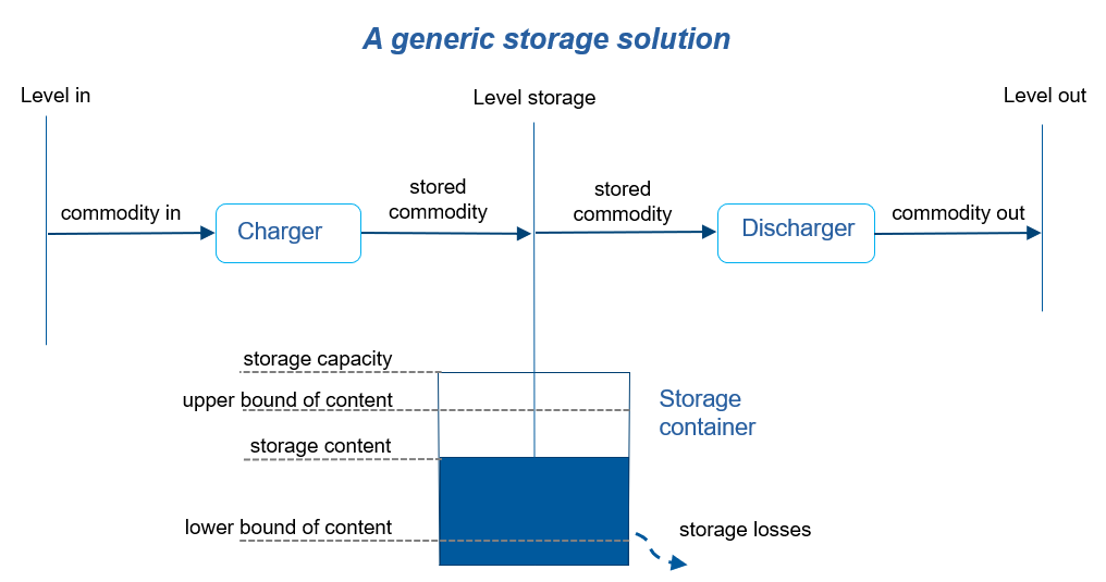
Storage section
Storage technologies can be used to store a commodity (e.g., water, heat, electricity, etc.) and shift it over sub-annual time slices. The storage solution presented here has three distinctive parts: (i) Charger: a technology for charging a commodity to the storage container, for example, a pump in a pumped hydropower storage (PHS) plant. (ii) Discharger: a technology to convert the stored commodity to the output commodity, e.g., a turbine in PHS. (iii) Storage container: a device for storing a commodity over time, such as a water reservoir in PHS.
Storage equations
The content of storage device depends on three factors: charge or discharge in one time step (represented by Equation STORAGE_CHANGE), the state of charge in the previous time step, and storage losses between two consecutive time steps.
Equation STORAGE_CHANGE
This equation shows the change in the content of the storage container in each sub-annual timestep. This change is based on the activity of charger and discharger technologies connected to that storage container. The notation \(S^{storage}\) represents the mapping set map_tec_storage denoting charger-discharger technologies connected to a specific storage container in a specific node and storage level. Where:
\(t^{C}\) is a charging technology and \(t^{D}\) is the corresponding discharger.
\(h-1\) is the time step prior to \(h\).
\[\begin{split}STORAGE\_CHARGE_{n,t,l,c,y,h} = \sum_{\substack{n^L,m,h-1 \\ y^V \leq y, (n,t^C,t,l,y) \sim S^{storage}}} output_{n^L,t^C,y^V,y,m,n,c,l,h-1,h} \cdot & ACT_{n^L,t^C,y^V,y,m,h-1} \\ - \sum_{\substack{n^L,m,c,h-1 \\ y^V \leq y, (n,t^D,t,l,y) \sim S^{storage}}} input_{n^L,t^D,y^V,y,m,n,c,l,h-1,h} \cdot ACT_{n^L,t^D,y^V,y,m,h-1} \quad \forall \ t \in T^{STOR}, & \forall \ l \in L^{STOR}\end{split}\]
Equation STORAGE_BALANCE
This equation ensures the commodity balance of storage technologies, where the commodity is shifted between sub-annual timesteps within a model period. If the state of charge of storage is set exogenously in one timestep through \(\storageinitial_{ntlcyh}\), the content from the previous timestep is not carried over to this timestep.
Equation STORAGE_BALANCE_INIT
Where \(\storageinitial_{ntlyh}\) has a non-zero value, this equation ensures that the amount of commodity stored at the end of the period is equal to that value plus any change during the period.
Equation STORAGE_EQUIVALENCE
This equation links \(\STORAGE\) to activity (\(\ACT\)) for each active storage container technology \(t\); this is distinct from the (dis)charge technologies \(t^C,t^D\) appearing in Equation STORAGE_CHANGE.